
Calculating likes on Instagram is not simple
The One-Liner That Takes 6 Months to Ship

It starts so innocently.
Product comes to you and says: “We need a like count on posts. Users tap a heart, we show the number. That’s it.”
You think about it for 30 seconds. A likes column in the posts table. An UPDATE posts SET likes = likes + 1 WHERE id = ? on every tap. Done. You could ship this before lunch.
But then the follow-up questions start.
“Actually, we also need likes per hour for trending. And likes by region for the analytics dashboard. And we need to detect like-spamming in real-time. Oh, and the feed ranking team wants a signal based on like velocity — likes per minute over the last 15 minutes — to boost viral content.”
Suddenly you’re not incrementing a counter. You’re computing time-windowed aggregations, sliding window rates, real-time anomaly detection, and multi-dimensional rollups — all on an event stream that peaks at 500K likes per second when a celebrity posts.
That UPDATE ... SET likes + 1 won’t survive the first traffic spike. Your Postgres instance will melt. You need to decouple ingestion from processing. You need to handle bursts without dropping events. You need to compute multiple aggregations on the same stream without duplicating infrastructure.
So you do what every senior engineer does in this situation. You open the architecture doc and write the sentence:
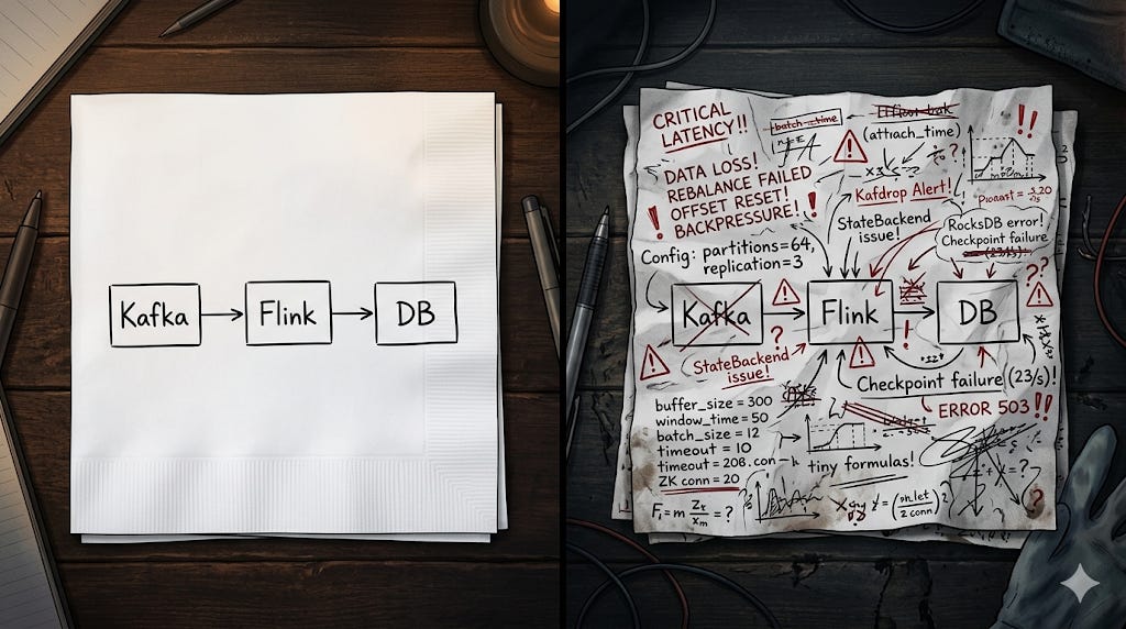
“Push like events to Kafka. Process them with Flink. Write aggregated data to DB.”
One line. Three components. Two arrows. Fits on a sticky note.
The architect nods. The tech lead approves. Someone creates a Jira epic with a 3-week estimate.
Six months later, you’re still shipping it.
Why This Escalation Is Inevitable
Here’s the thing most people miss: the problem was never “count likes.” The problem was “count likes at scale, in real time, for multiple consumers, with correctness guarantees, while the world is on fire.”
Every real-world feature that starts as a simple counter eventually needs these properties: durability (don’t lose events), scalability (handle 100x traffic spikes), flexibility (multiple downstream consumers computing different things from the same stream), and timeliness (results in seconds, not minutes).
No single database query gives you all four. That’s why you end up with a streaming architecture. Not because engineers love complexity, but because the requirements demand it.
The Kafka-Flink-DB pattern is the industry’s answer to this exact class of problem. And on a whiteboard, it looks clean. Elegant, even.
But every box in that diagram hides a month of decisions. Every arrow hides a class of failure modes. And the spaces between the boxes? That’s where production incidents live.
Let me walk you through what actually happens when you try to build this. Not the tutorial version. The production version. The one that has to work at 3 AM when your on-call engineer is asleep.
Part 1: “Push Messages to Kafka”
Four words. Dozens of decisions.
Choosing a Serialization Format
Your producers need to serialize data before pushing to Kafka. You have three mainstream options: JSON, Avro, and Protobuf.
JSON is what everyone starts with because it’s human-readable and requires zero setup. But JSON has no schema enforcement. Your producer can send {"user_id": "abc123"} today and {"userId": "abc123"} tomorrow. Different field name. No warning. Your downstream consumer breaks silently — it doesn’t crash, it just starts writing nulls into your database. You find out three days later when a dashboard goes blank.
Avro solves this with a schema registry. Every message is serialized against a registered schema, and the registry enforces compatibility rules. If a producer tries to remove a required field or change a type, the registry rejects the schema update before a single bad message hits the topic. The tradeoff? Now you’re running another piece of infrastructure. The Confluent Schema Registry is effectively a stateful service backed by a Kafka topic (_schemas). It needs to be highly available, because if the registry goes down, producers can’t serialize and consumers can’t deserialize. You’ve added a new single point of failure to your pipeline.
Protobuf gives you similar guarantees with smaller payloads (roughly 30-40% smaller than Avro for the same data, depending on field types). The catch is that Protobuf schemas are defined in .proto files that need to be compiled into language-specific code. This introduces a build-time dependency. Every schema change requires regenerating code, updating libraries, and redeploying both producers and consumers. In a microservices environment with 15 teams, coordinating proto changes becomes its own project.
There’s no “right” answer. But the choice you make in week one shapes your operational life for years.
Partition Strategy
Kafka topics are split into partitions. Partitions are the unit of parallelism — each partition is consumed by exactly one consumer in a consumer group. More partitions means more consumers can work in parallel.
Sounds simple. Just crank up the partition count, right?
Not quite. The number of partitions has second-order effects that most tutorials skip.
Every partition has a leader replica on one broker and follower replicas on others. When a broker goes down, Kafka needs to elect new leaders for every partition that broker was leading. If you have 10,000 partitions spread across 5 brokers, a single broker failure triggers ~2,000 leader elections. During this window (which can last seconds to minutes depending on your configuration), those partitions are unavailable for writes.
There’s also the consumer rebalance problem. When a consumer joins or leaves the group, Kafka reassigns partitions across all consumers. With the default “eager” rebalance protocol, this means every consumer stops processing, gives up all its partitions, and waits for new assignments. With 1,000 partitions, the rebalance can take 30-60 seconds during which zero messages are being processed. There are cooperative rebalance protocols (like CooperativeStickyAssignor) that reduce this pain, but they add complexity and have their own edge cases around revocation.
The real art is choosing the partition key. This determines which messages land on which partition. Get it wrong and you’ve got hot partitions — one partition receiving 80% of the traffic while others sit idle. This is especially brutal when your key has a skewed distribution (think: a partition key based on country, where 40% of your traffic comes from the US).
Durability vs. Throughput
The acks configuration on your producer controls how many broker acknowledgments are required before a write is considered successful.
acks=1 means only the leader broker needs to confirm. Fast, but if the leader dies before replicating to followers, that data is gone.
acks=all means every in-sync replica must confirm. Durable, but your write latency increases by the time it takes the slowest follower to write. On a cross-rack deployment, this can add 5-15ms per write.
And then there’s the min.insync.replicas setting, which determines how many replicas must be in-sync for a acks=all write to succeed. If you set replication factor to 3 and min.insync.replicas to 2, you can tolerate one replica being down while still guaranteeing durability. But if two replicas go down, your producer starts getting NotEnoughReplicasException and your pipeline stalls. You’ve traded data loss for availability loss.
Most production systems set acks=all with min.insync.replicas = replication_factor - 1. But “most” doesn’t mean all. High-throughput analytics pipelines where losing a few events is acceptable often use acks=1 with higher batch sizes and compression — because when you’re processing clickstream data at 2 million events per second, the 10ms of extra latency from acks=all multiplied across millions of messages adds up to real throughput reduction.
Schema Evolution
Your pipeline has been running for 6 months. Now the product team wants to add a device_type field to your event. Sounds trivial.
But you have three months of historical data in Kafka (you set retention to 90 days for replay capability). Your new consumers need to read both old messages (without device_type) and new messages (with device_type). Your old consumers, which haven’t been redeployed yet, need to read new messages without crashing.
This is the schema evolution problem, and it’s where things get subtle.
With Avro and a schema registry, you set compatibility modes. Backward compatibility means new consumers can read old data. Forward compatibility means old consumers can read new data. Full compatibility means both. Adding an optional field with a default value is backward compatible. Removing a field is forward compatible. Renaming a field is neither — it’s a breaking change.
Without a schema registry (which is most teams starting out with JSON), schema evolution is managed by convention and prayer. You add the field, hope every consumer handles the null case, and discover the ones that don’t when they crash in production.
Part 2: “Process Them with Flink”
This is where the real complexity lives.
Event Time vs. Processing Time
Flink gives you a choice: do you process events based on when they were created (event time) or when Flink receives them (processing time)?
Processing time is simpler to implement but produces incorrect results under any real-world condition. Here’s why.
Imagine you’re computing hourly aggregations. Your pipeline has 10 minutes of consumer lag (not uncommon during a traffic spike). An event created at 2:55 PM arrives at Flink at 3:05 PM. With processing time, this event lands in the 3:00-4:00 PM window. Your 2:00-3:00 PM window is undercounted. Your 3:00-4:00 PM window is overcounted. Your aggregations are wrong, and you won’t know until someone compares them against the source of truth (if one exists).
Event time fixes this by using the timestamp embedded in the event itself. But event time introduces a different problem: Flink needs to know when it’s “safe” to close a window. If you’re aggregating 2:00-3:00 PM events, how does Flink know when all 2:00-3:00 PM events have arrived? What if there’s a producer that’s 30 seconds behind? What if a network partition delayed events by 5 minutes?
This is the watermark problem.
Watermarks
A watermark is Flink’s way of saying “I believe all events with a timestamp before X have arrived.” When the watermark passes the end of a window, Flink fires the window computation and emits results.
You configure watermarks with a bounded-out-of-orderness strategy. forBoundedOutOfOrderness(Duration.ofSeconds(30)) tells Flink to wait 30 seconds past the window end before firing. This handles most late-arriving events.
But how do you choose that duration?
Too aggressive (say, 5 seconds) and you drop a meaningful percentage of late events. They arrive after the watermark has passed, the window has already fired, and by default they’re silently discarded. You can route them to a side output for separate handling, but now you need a reconciliation pipeline on top of your main pipeline.
Too lenient (say, 5 minutes) and your results are delayed by 5 minutes. For a real-time dashboard, that defeats the purpose. Your users are looking at data that’s 5 minutes stale, and they’re asking why they’re using a “real-time” pipeline at all.
And here’s the part that really hurts: the right watermark duration isn’t constant. It varies by source, by time of day, by traffic pattern. During peak hours with healthy producers, 10 seconds might be fine. During an incident where a producer is buffering events, you might need 2 minutes. A static watermark configuration is always wrong — it’s just a question of how wrong, and when.
Some teams implement dynamic watermarks that adjust based on observed event-time skew. This works, but adds significant operational complexity. You’re now monitoring and tuning an adaptive parameter that directly affects the correctness of your output.
State Management
Flink is a stateful stream processor. When you compute a windowed aggregation, Flink maintains the accumulated state (partial sums, counts, min/max values) for every active window, for every key, in memory.
Let me make that concrete. Say you’re aggregating events by user_id over 1-hour tumbling windows. You have 10 million active users. Each window state holds a counter and a sum — let’s say 100 bytes per key. That’s 1 GB of state per window. But Flink might have multiple windows active simultaneously (the current hour, plus late-arriving events for the previous hour). Now you’re at 2 GB. Add a sliding window with a 5-minute slide for your alerting pipeline, and you’ve got 12 overlapping windows per hour. Your state is now 12 GB.
This state is stored in a state backend. Flink’s default is the HashMapStateBackend, which keeps everything on the JVM heap. Fast, but you’re limited by available memory and subject to GC pauses (which can be catastrophic for a streaming application — a 10-second GC pause means 10 seconds of no processing, which cascades into backpressure, consumer lag, and potential rebalances).
The production choice is usually RocksDB as the state backend, which spills to disk. But RocksDB brings its own tuning nightmare. You’re now configuring block cache sizes, write buffer counts, max background compactions, bloom filter settings, and compaction strategies — inside a streaming framework. Most Flink engineers I know spend more time tuning RocksDB than tuning Flink itself.
Checkpointing
Flink achieves fault tolerance through periodic checkpoints. A checkpoint is a consistent snapshot of all operator state, saved to remote storage (usually S3 or HDFS).
During a checkpoint, Flink injects barrier markers into the data stream. When an operator receives a barrier on all its input channels, it snapshots its state and forwards the barrier. This is the Chandy-Lamport algorithm — it’s elegant in theory.
In practice, checkpoint performance is one of the top operational challenges in Flink.
If your state is 50 GB and your checkpoint interval is 60 seconds, you’re pushing 50 GB to S3 every minute. That’s sustained throughput of ~850 MB/s to your checkpoint storage. Flink does incremental checkpoints (only uploading changed state since the last checkpoint), which helps, but for high-throughput applications the checkpoint overhead is real.
If a checkpoint takes longer than the checkpoint interval, you have a problem. Checkpoints start backing up. Flink’s checkpoint coordinator begins aborting timed-out checkpoints. If no checkpoint succeeds for an extended period and the application fails, recovery goes back to the last successful checkpoint — which could be 10 or 20 minutes old. That means reprocessing 10-20 minutes of data from Kafka, which triggers a burst of writes to your sink, which might overwhelm your database.
Checkpoint alignment is another subtlety. When an operator receives a barrier on one input channel but not another, it either buffers records from the faster channel (aligned checkpoints — preserves exactly-once but increases latency) or processes them without waiting (unaligned checkpoints — reduces latency but increases checkpoint size because in-flight records are included in the snapshot).
The Backpressure Death Spiral
This is the failure mode that catches teams off guard.
Your sink (the database write) slows down. Maybe the DB is under load, maybe a disk is degrading. The Flink sink operator can’t write fast enough, so it stops pulling from the upstream operator. Flink’s backpressure mechanism kicks in: upstream operators slow down to match the slowest downstream operator. This propagates all the way to the Kafka source operator.
The Kafka source stops fetching records. From Kafka’s perspective, this consumer has stopped consuming. If the consumer doesn’t send a heartbeat within session.timeout.ms (default 45 seconds), the consumer group coordinator declares it dead and triggers a rebalance. The rebalance reassigns partitions, which causes Flink to pause, reinitialize its Kafka consumers, and seek to the correct offsets. This takes time. During this time, lag increases further. When processing resumes, Flink tries to catch up, pushing even more load to the already struggling sink. The sink slows down more. More backpressure. More rebalances.
This is the death spiral. I’ve seen it take down production pipelines for hours.
The mitigation involves multiple coordinated settings: increasing session.timeout.ms and max.poll.interval.ms on the Kafka consumer side, implementing circuit breakers or rate limiting on the sink side, setting up backpressure monitoring with alerts that fire before things cascade, and having a runbook for manual intervention (like temporarily diverting sink writes to a buffer).
Part 3: “Write Aggregated Data to DB”
The last arrow on the whiteboard. Deceptively simple.
Choosing the Right Database
This choice depends entirely on your query patterns, and most teams don’t think about it deeply enough until they’re already in trouble.
Postgres can handle maybe 10-20K writes per second on a well-tuned instance with SSDs. That sounds like a lot until your pipeline is emitting 100K aggregated records per second during peak. You start connection pooling with PgBouncer, which helps, but you’re still single-node. You shard, which gives you write throughput but makes cross-shard queries painful.
Cassandra handles high write throughput beautifully — 100K+ writes per second per node, linear scalability by adding nodes. But Cassandra’s query model is fundamentally different from SQL. You design your tables around your queries, not your data model. Want to query by user_id? That’s one table. Also want to query by timestamp range? That’s a second table with the same data, different partition key. You’re maintaining multiple materialized views of the same data, paying the storage cost and the write amplification.
ClickHouse is increasingly the answer for analytical workloads — column-oriented, fast for aggregation queries, excellent compression. But ClickHouse doesn’t support transactions, updates are expensive (it’s an append-only columnar store), and its replication model is more operationally complex than Postgres.
Time-series databases like TimescaleDB or InfluxDB work well when your data is strictly time-ordered, but struggle with high-cardinality dimensions (like aggregating by user_id when you have 50 million users).
There’s also the increasingly common pattern of using multiple stores: Redis for hot data (last hour, sub-10ms reads), a columnar store like ClickHouse or Druid for medium-term analytical queries, and something like S3 + Parquet for long-term storage. But now you’ve tripled your sink complexity. Flink needs to write to three places instead of one. Each sink has its own failure modes, its own backpressure characteristics, its own consistency guarantees.
Idempotency
This is the one thing that, if you get wrong, corrupts your data.
Flink processes each event at least once. During failure recovery, Flink replays events from the last successful checkpoint. This means your sink will see duplicate writes. If your sink is a simple INSERT, you’ll double-count.
The fix is making your writes idempotent. Instead of INSERT INTO metrics (key, count) VALUES ('foo', 5), you use INSERT INTO metrics (key, count) VALUES ('foo', 5) ON CONFLICT (key) DO UPDATE SET count = 5. The write produces the same result whether it’s executed once or five times.
But idempotency gets complicated with aggregations. If you’re computing a running sum, you can’t just upsert the latest value — you need to know which checkpoint epoch produced which value. Some teams embed a checkpoint ID in their writes and deduplicate on that. Others use Flink’s two-phase commit protocol with databases that support it (Postgres with XA transactions, for example). The two-phase commit approach gives you true exactly-once semantics end-to-end, but the coordination overhead reduces your maximum throughput by 20-40%.
Connection Management
Your Flink job runs with, say, 64 parallel sink tasks. Each task opens a connection to the database. That’s 64 connections. If you’re running two Flink jobs (one for real-time and one for backfill), that’s 128. Add connection overhead from your application servers, and your database’s connection pool is saturated.
Postgres has a default connection limit of 100. You’ll hit this in the first week. PgBouncer helps but introduces its own configuration (transaction vs. session pooling, pool sizing, timeout tuning). Cassandra handles connections better by design, but even Cassandra has per-node connection limits that you’ll hit at scale.
The subtler issue is connection lifecycle management. Database connections fail. Networks hiccup. When a sink task’s connection dies, does it retry? How many times? With what backoff? Does it fail the entire Flink job (triggering a full restart from checkpoint) or just that one task? The default behavior in most Flink sink connectors is to throw an exception that fails the entire job. A single connection timeout can restart your entire pipeline, which then needs to recover state, replay from Kafka, and catch up on the accumulated lag.
Batching
Writing one record at a time to a database is comically inefficient. Network round trips, transaction overhead, and write amplification make single-record writes 10-100x slower than batched writes.
But batching introduces latency. If you batch 1,000 records before writing, and your throughput is 100 records per second, that’s a 10-second delay. Your “real-time” pipeline is now 10 seconds behind.
The standard approach is to batch by size OR time — flush when you hit 1,000 records or 5 seconds, whichever comes first. But this interacts with checkpointing in non-obvious ways. If Flink takes a checkpoint while your sink has a half-full batch that hasn’t been flushed, that data is in limbo. On recovery, Flink replays from the checkpoint, and those records get processed again. If your sink flushed the batch before the checkpoint completed, you’ve double-written. If it didn’t flush, you’ve lost those records until replay catches up.
Flink handles this correctly if you implement the CheckpointedFunction interface and flush your buffer during checkpoint snapshotting. But this is a common source of bugs in custom sinks.
The Operational Iceberg
Here’s what I haven’t even covered yet — monitoring, alerting, deployment, and the day-to-day operational work that makes this pipeline actually reliable.
You need to monitor consumer lag per partition (not just per topic — a single lagging partition indicates a hot key or a slow consumer task). You need to monitor Flink’s checkpoint duration, checkpoint size, and checkpoint failure rate. You need to monitor backpressure per operator. You need to monitor your sink’s write latency at P99, not just average.
You need alerts that fire early enough to intervene before a cascading failure. A good starting point: alert on checkpoint duration exceeding 80% of checkpoint interval, alert on consumer lag exceeding 2x your watermark duration, alert on sink P99 latency exceeding 5x baseline.
You need a deployment strategy. Flink jobs are long-running. You can’t just deploy a new version and restart — that triggers a full recovery from checkpoint. Flink supports savepoints (manual, portable checkpoints) that let you stop a job, deploy a new version, and resume from where you left off. But savepoints have compatibility requirements: you can’t change the parallelism, operator chain, or state schema without migration steps.
You need a playbook for what to do when Kafka goes into under-replicated partition state, when Flink runs out of heap and OOMs, when your database’s disk fills up because write throughput exceeded your retention policy.
The Real Architecture
So let’s look at what that one-liner actually translates to in production.
Ingestion layer: Schema registry, serialization library, producer tuning (batch size, linger.ms, compression, acks), topic configuration (partitions, replication, retention), monitoring for producer errors and broker health.
Processing layer: Flink cluster (JobManager, TaskManagers, resource management), watermark strategy, window configuration, state backend tuning (RocksDB or heap), checkpoint configuration (interval, timeout, storage, incremental vs. full), backpressure monitoring, metrics export (Prometheus + Grafana), JVM tuning (GC, heap, metaspace).
Sink layer: Database selection, connection pooling, batching strategy, idempotency logic, exactly-once protocol (optional), error handling and retry policy, schema management on the DB side.
Operations layer: Consumer lag monitoring, checkpoint health monitoring, backpressure alerts, deployment automation with savepoints, incident runbooks, capacity planning, cost tracking.
That’s four full layers of infrastructure, each with its own failure modes, tuning parameters, and operational procedures.
So Why Does Anyone Build This?
Because when you get it right, it’s incredibly powerful.
A well-tuned Kafka-Flink pipeline can process millions of events per second with sub-second latency and exactly-once guarantees. It can handle traffic spikes without dropping data, recover from failures without human intervention, and scale horizontally by adding partitions and Flink task slots.
The problem isn’t that the architecture is bad. The problem is that the whiteboard version doesn’t communicate 10% of what’s actually involved. Teams that treat it as a “straightforward integration project” end up learning these lessons one production incident at a time.
The architecture diagram fits on a napkin. The operational reality fills a runbook.
If you’re building a pipeline like this, budget for the complexity. Staff for the operations. And the next time someone points to three boxes and two arrows and says “it’s simple” — send them this article.
If this piece gave you a new appreciation for what “just use Kafka and Flink” actually means, share it with your team. The engineer who’s about to build this pipeline will thank you.
Follow me for more deep dives where I take apart the engineering that hides behind simple architecture diagrams.
You articles are so goated sir.
The curious thing about this type of article is that its popularity is sometimes inversely proportional to its level of complexity and quality. Few likes here, but who else will be interested in this besides a small, select group of readers?